
Optimizing price, maximizing revenue
Published:
Setting a right price of products/services is one of the most important decisions a business can make. Under-pricing (and over-pricing) can hurt a company’s bottom line. Two determinants/indicators of business revenue are product prices and quantity sold. At higher price revenue is expected to be higher, if quantity sold is constant. However we know from our everyday experience that price and quantity are inversely related – as the price of something goes up, people show less intent to buy it.
The opposite is also true, that is, as price goes down, sales go up (that’s why we big “sale” events in shopping malls round the year). But that doesn’t mean that the revenue will always go up.
So an important question to ask is: if higher price means sales down and at lower price revenue goes down then where is the sweet spot, the right price, that maximizes revenue? With a simple example we’ll examine how to optimization price to maximize revenue and profit.
Import libraries
from __future__ import print_function
import numpy as np
import pandas as pd
from pandas import DataFrame
import matplotlib.pyplot as plt
import seaborn as sns
import statsmodels.api as sm
from statsmodels.compat import lzip
from statsmodels.formula.api import ols
%matplotlib inline
Data
Data in this analysis comes from here [Susan Li has a nice blog post about price elasticity of demand (i.e. sensitivity of demand to change in price) explained using the same dataset]. This is a time series, quarterly dataset of beef sales (quantity) and corresponding price.
This dataset will be used first to find price elasticity of demand and then to find at what price the profit is maximized.
# Load data
beef = pd.read_csv('https://raw.githubusercontent.com/susanli2016/Machine-Learning-with-Python/master/beef.csv')
# View first few rows
beef.tail(5)
| Year | Quarter | Quantity | Price | |
|---|---|---|---|---|
| 86 | 1998 | 3 | 17.5085 | 277.3667 |
| 87 | 1998 | 4 | 16.6475 | 279.5333 |
| 88 | 1999 | 1 | 16.6785 | 278.0000 |
| 89 | 1999 | 2 | 17.7635 | 284.7667 |
| 90 | 1999 | 3 | 17.6689 | 289.2333 |
Step 1: Define the profit function
We know,
profit = revenue - cost (1)
We also know,
revenue = qt_demanded * price (2)
Therefore,
profit = qt_demanded * price - cost (3)
Step 2: Define the demand function
Assuming that the cost is constant, we first need to estblish the relationship between qt_demanded and price:
qt_demanded = f(price) (4)
This demand function can be estimated based on hitorical price and corresponding sales data.
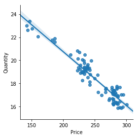
# demand curve estimation
sns.lmplot( x="Price", y="Quantity", data=beef, fit_reg=True, size=4)
<seaborn.axisgrid.FacetGrid at 0x195b918df60>
# fit OLS model
model = ols("Quantity ~ Price", data=beef).fit()
# print model summary
print(model.summary())
                            OLS Regression Results
==============================================================================
Dep. Variable:               Quantity   R-squared:                       0.901
Model:                            OLS   Adj. R-squared:                  0.900
Method:                 Least Squares   F-statistic:                     811.2
Date:                Thu, 18 Apr 2019   Prob (F-statistic):           1.69e-46
Time:                        15:51:26   Log-Likelihood:                -77.493
No. Observations:                  91   AIC:                             159.0
Df Residuals:                      89   BIC:                             164.0
Df Model:                           1
Covariance Type:            nonrobust
==============================================================================
                 coef    std err          t      P>|t|      [0.025      0.975]
------------------------------------------------------------------------------
Intercept     30.0515      0.413     72.701      0.000      29.230      30.873
Price         -0.0465      0.002    -28.482      0.000      -0.050      -0.043
==============================================================================
Omnibus:                        3.453   Durbin-Watson:                   1.533
Prob(Omnibus):                  0.178   Jarque-Bera (JB):                2.460
Skew:                           0.237   Prob(JB):                        0.292
Kurtosis:                       2.349   Cond. No.                     1.74e+03
==============================================================================

Warnings:
[1] Standard Errors assume that the covariance matrix of the errors is correctly specified.
[2] The condition number is large, 1.74e+03. This might indicate that there are
strong multicollinearity or other numerical problems.
Step 3: Parameterize the profit function in step 1
The demand function with parameter values coming from the above regression:
    qt_demanded=30.05-0.0465*price (5) Therefore, the profit function in equation (3) becomes

    profit = (30.05-0.0465*price)*price - cost (6)
Step 4: Finding the price that maximizes profit
Price = [320, 330,340,350, 360, 370, 380, 390] # a range of diffferent prices to find the optimum one
Cost = 80 # a fixed cost in this case
Revenue = []
for i in Price:
    quantity_demanded=30.05-0.0465*i
    Revenue.append((i-cost)*quantity_demanded) # profit function

# create data frame of price and revenue
profit=pd.DataFrame({"Price": Price, "Revenue": Revenue})
#plot revenue against price
plt.plot(profit["Price"], profit["Revenue"])
[<matplotlib.lines.Line2D at 0x195ba1cf9b0>]
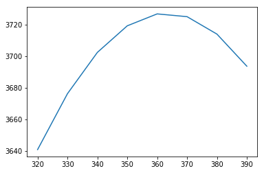
# price at which the revenue is maximum
profit[profit['Revenue'] == profit['Revenue'].max()]

#profit.loc[profit['Revenue'].idxmax()]
| Price | Revenue | |
|---|---|---|
| 4 | 360 | 3726.8 |
So USD 360 is the price, from a lis tof prices, at which the profit is maximized. We used a price interval of USD 10, this could be any number that gives the right outcome.