Spatial data visualization with tidycensus
Published:
Location! Location!! Location!! The location people live in tells us a lot about the space itself as well as the people who live in there. This demo is about spatial data visualization with tidycensus R package with two variables of interest – population and race distribution. First we will get the big picture at the Virginia state scale, then will zoom in on northern Virginia in Washington DC metro area.
Tools
We do not have to start from scratch. As always the case, someone has already done the hard work for us so we can stand on their shoulders.
Kyle Walker in this case has developed an rstat package called tidycensus. This package allows for easy access, analysis and visualization of Census Beureau data on hundreds of variables.
Not that in Python you can not do spatial analysis/visualization of census data, but certainly not as easily as in R because of some excellent rstats packages available and tailored for this purpose.
To be able to use tidycensus you’ll need your own Census API Key. If you do not have one, get one.
The only other library you’ll need is tidyverse; and this is it! If you like interactive visialization of maps (i.e. zoom in zoom out etc.) you will need additional libraries and codes.
Okay, so here we go …
# import libraries
library(tidycensus)
library(tidyverse)
options(tigris_use_cache = TRUE)

# get your Census Bureau API key
census_api_key("API_KEY_HERE")
To install your API key for use in future sessions, run this function with `install = TRUE`.
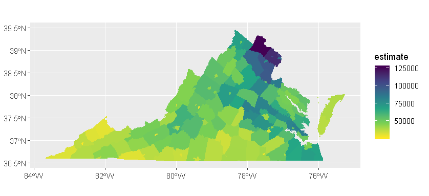
# geting VA population data of counties
vapop <- get_acs(state = "VA", geography = "county",
                  variables = "B19013_001", geometry = TRUE)
# plot VA population
vapop %>%
  ggplot(aes(fill = estimate)) +
  geom_sf(color = NA) +
  coord_sf(crs = "+init=epsg:4326") + # original 26911
  scale_fill_viridis_c(option = "viridis", direction=-1) #  original: scale_fill_viridis_c(option = "magma")
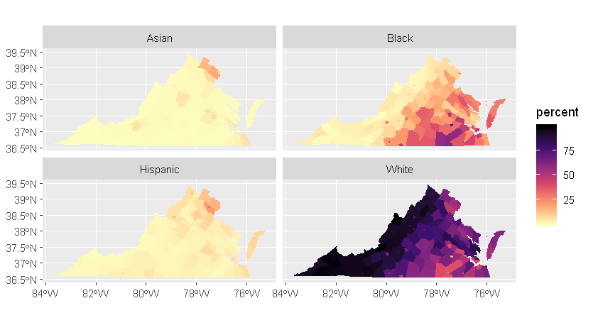
# specify races
races <- c(White = "P005003",
              Black = "P005004",
              Asian = "P005006",
              Hispanic = "P004003")

# get decennial data on races
varace <- get_decennial(geography = "county", variables = races,
                  state = "VA", geometry = TRUE,
                  summary_var = "P001001")

# plot race variables as a percent of total population
varace %>%
  mutate(percent = 100 * (value / summary_value)) %>% # create a calculated column of percent value
  ggplot(aes(fill = percent)) +
  facet_wrap(~variable) +
  geom_sf(color = NA) +
  coord_sf(crs = "+init=epsg:4326") +
  scale_fill_viridis_c(option = "magma", direction=-1)
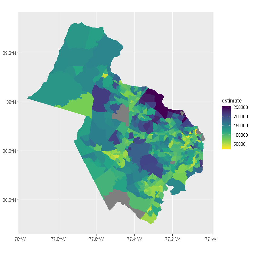
Zooming in on Northern Virginia
# specify counties that constitute Northern Virginia
NOVA = c("Fairfax County", "Fairfax City", "Manassas Park City", "Arlington County", "Loudoun County", "Alexandria City", "Falls Church City", "Prince William County", "Manassas City")

# get population data of NOVA cunties
novapop <- get_acs(state = "VA", county = NOVA, geography = "tract",
                  variables = "B19013_001", geometry = TRUE)

# plot NOVA population

novapop %>%
  ggplot(aes(fill = estimate)) +
  geom_sf(color = NA) +
  coord_sf(crs = "+init=epsg:4326") +
  scale_fill_viridis_c(option = "viridis", direction=-1) #  original: scale_fill_viridis_c(option = "magma")
# get decennial data on races
novarace <- get_decennial(geography = "tract", variables = races,
state = "VA", county = NOVA, geometry = TRUE,
summary_var = "P001001")
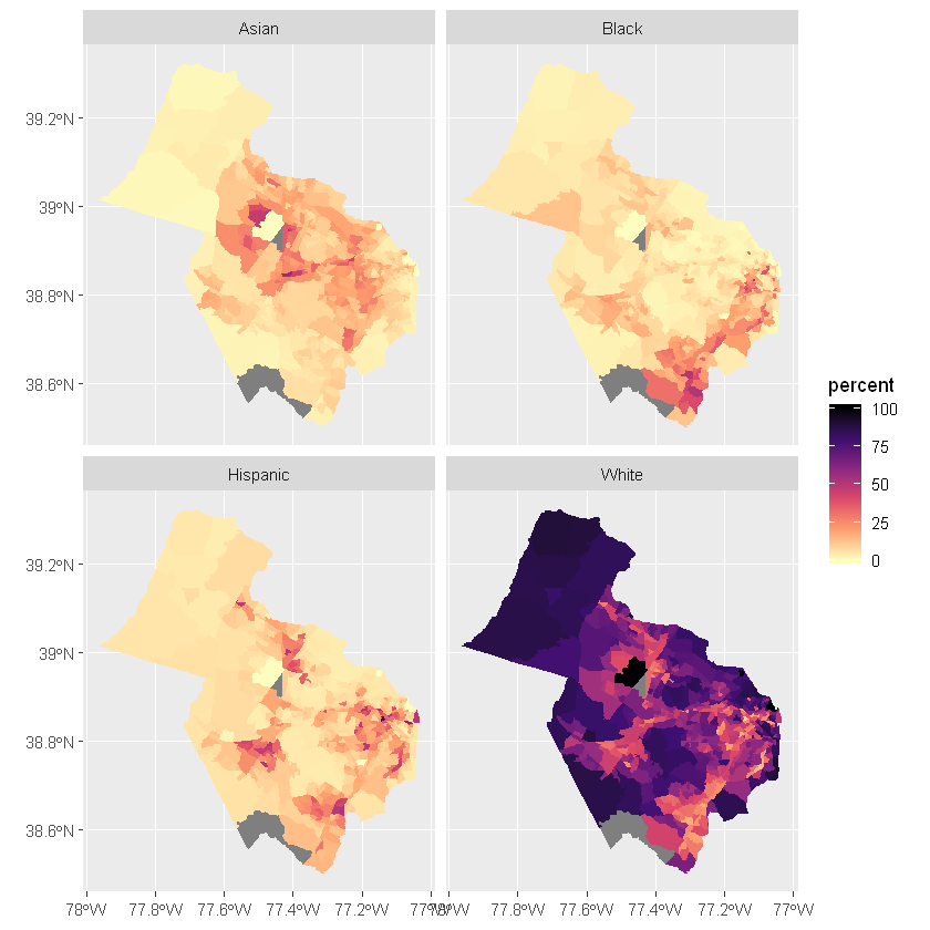
# plot race variables as a percent of total population
novarace %>%
mutate(percent = 100 * (value / summary_value)) %>% # create a calculated column of percent value
ggplot(aes(fill = percent)) +
facet_wrap(~variable) +
geom_sf(color = NA) +
coord_sf(crs = "+init=epsg:4326") +
scale_fill_viridis_c(option = "magma", direction=-1)